Descriptor analysis/Coarse-graining

Warning

The following procedures and analyses should be considered experimental. They are not well-tested and there is no related peer-reviewed publication.

This short tutorial shows how to prepare and run a descriptor analysis which can be useful when creating a coarse-grained (CG) model based on neural network potentials. The steps outlined here correspond to the subfolders of the examples/coarse-graining directory in the repository. The descriptor analysis itself is described in detail inside the Jupyter notebook step-3_cluster-analysis/analyze-descriptors.ipynb.

Note

The tools nnp-atomenv and nnp-scaling need to be compiled to follow the steps presented in this tutorial.

Step 0 (optional): Coarse-grained data set

Note

This step is optional, the descriptor analysis may also yield insights if applied directly to the full, atomistic description of the system.

First, we need to create a data set which contains the coarse-grained description of the original structures. In the example (directory step-0_cg-data-set) we start with a data set of bulk water (input.data) where we apply the following coarse-graining strategy: for each oxygen atom we identify the two closest hydrogen neighbors and compute then the center of mass coordinates of all molecules via

\[\vec{R} = \vec{r}_O - \frac{2 m_H \left(\Delta \vec{r}_{OH_1} + \Delta \vec{r}_{OH_2} \right)}{m_O + 2 m_H},\]

where \(\Delta \vec{r}_{jk} = \vec{r}_j - \vec{r}_k\). The force acting on the center of mass is then just the sum of all forces in each molecule.

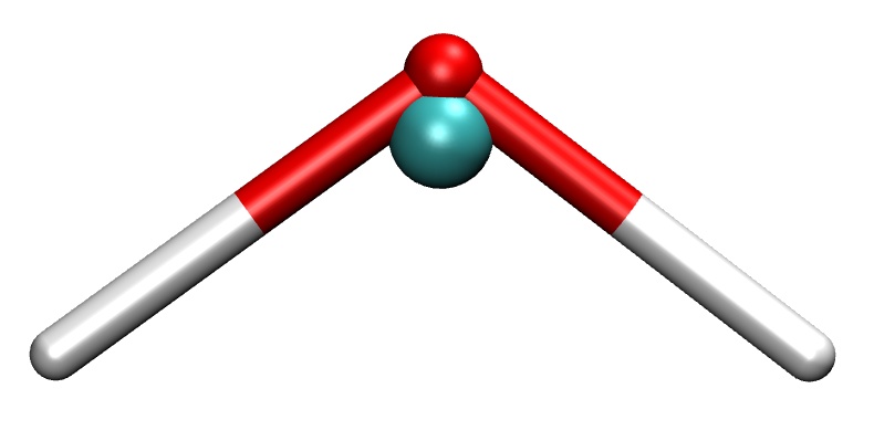
Water molecule with center of mass position. — A water molecule and its coarse-grained (center of mass) representation (turquoise sphere).

An example C++ code is provided to perform this conversion in nnp-cgdata.cpp making use of the libnnp library. To build the executable just run make (libnnp needs to be compiled beforehand in the main src directory). Then run the executable with an appropriate cutoff radius for the neighbor list as the only argument:

./nnp-cgdata 2.3

Here, we use a cutoff of 2.3 bohr which ensures that the two closest hydrogen neighbors are found for each oxygen atom. This will create the file output.data which contains the desired coarse-grained center of mass particles representing the water molecules.

Hint

The “element symbol” of the CG particles in this example is Cm. Normally, this would correspond to the element Curium but here we use it to abbreviate “center of mass”.

The nnp-cgdata.cpp code demonstrates the usage of the C++ API to manipulate datasets of configurations. Of course such a task can also be performed with external software.

Step 1: Create symmetry function set

This step is common to regular NNP training with n2p2: for a given data set we need to prepare an appropriate symmetry function set and compute the scaling data. Please see also this section for further information. For this example, an input.nn file is already prepared in step-1_scaling-data which contains symmetry function definitions for our coarse-grained description of water:

...
symfunction_short Cm 2 Cm 0.30  4.0 12.00
symfunction_short Cm 2 Cm 0.60  4.0 12.00
symfunction_short Cm 2 Cm 1.50  4.0 12.00
symfunction_short Cm 3 Cm Cm 0.03  1.0 1.0   12.00000
symfunction_short Cm 3 Cm Cm 0.03 -1.0 1.0   12.00000
...

Together with the data set file input.data (file is provided, it is the output.data of step 0 above) we can proceed to compute the symmetry functions statistics:

mpirun -np 4 ../../../bin/nnp-scaling 500

We can safely ignore (or delete) the output files sf.???.????.histo, we only require the scaling.data file for the next steps.

Step 2: Generate atomic environment data

Next, in order to feed the descriptor analysis Jupyter notebook in the final step, we need to prepare atomic environment data for our system. Please read the description of the tool nnp-atomenv for a detailed explanation how this data is constructed. The required files from the previous steps are prepared in the step-2_atomic-env directory. For the coarse-graining example we use the command

../../../bin/nnp-atomenv 500 4

where the second argument determines the maximum number of neighbor particles considered for the atomic environment data. Again, we can ignore all output files except atomic-env.dGdx which we use in the final step.

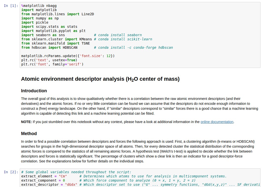
Step 3: Analyze descriptors

Finally, everything is ready to start the Jupyter notebook analyze-descriptors.ipynb which carries out the actual descriptor analysis. The notebook and necessary files are provided in step-3_cluster-analysis. After starting Jupyter with

jupyter notebook analyze-descriptors.ipynb

we can run all cells which may take a while. All further steps of the descriptor analysis are described in the notebook’s comment cells.